Full-Volume Instance Segmentation

This tutorial demonstrates the complete topo pipeline on a single volume (no tiling):

1. Create synthetic instance data

2. Generate diffusion flows

3. Postprocess flows into instance labels

4. Visualize every intermediate step

1. Create Synthetic Data

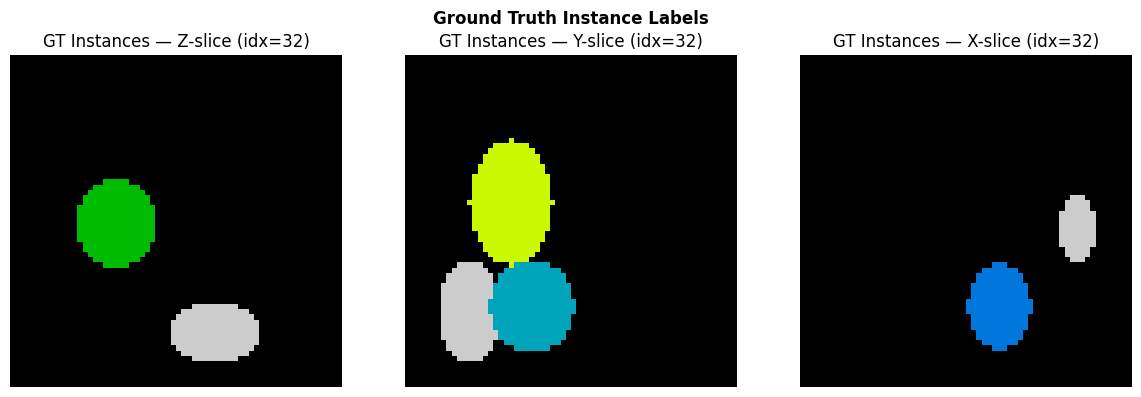
We generate a small 64x64x64 volume with 4 non-overlapping ellipsoidal instances of varying sizes and aspect ratios — mimicking organelles like mitochondria.

import numpy as np
import matplotlib.pyplot as plt

def make_synthetic_instances(shape=(64, 64, 64), n_instances=4, seed=42):
    """Create a volume with non-overlapping ellipsoidal instances."""
    rng = np.random.RandomState(seed)
    vol = np.zeros(shape, dtype=np.int32)
    coords = np.mgrid[0:shape[0], 0:shape[1], 0:shape[2]].astype(np.float32)

    for inst_id in range(1, n_instances + 1):
        # Random center (away from edges)
        margin = 10
        center = [rng.randint(margin, s - margin) for s in shape]
        # Random semi-axes (elongated)
        radii = [rng.randint(5, 15) for _ in range(3)]

        # Ellipsoid mask
        dist = sum(
            ((coords[ax] - center[ax]) / radii[ax]) ** 2
            for ax in range(3)
        )
        mask = dist <= 1.0

        # Only place where empty
        mask = mask & (vol == 0)
        vol[mask] = inst_id

    return vol

gt_instances = make_synthetic_instances()
n_inst = len(np.unique(gt_instances[gt_instances > 0]))
print(f"Volume shape: {gt_instances.shape}")
print(f"Instances: {n_inst}")

Volume shape: (64, 64, 64)
Instances: 4

# Visualize the ground truth — middle Z-slice
fig, axes = plt.subplots(1, 3, figsize=(12, 4))
for ax, (axis, title) in zip(axes, [(0, "Z-slice"), (1, "Y-slice"), (2, "X-slice")]):
    mid = gt_instances.shape[axis] // 2
    slc = [slice(None)] * 3
    slc[axis] = mid
    axes_img = gt_instances[tuple(slc)]
    ax.imshow(axes_img, interpolation="nearest", cmap="nipy_spectral")
    ax.set_title(f"GT Instances — {title} (idx={mid})")
    ax.axis("off")
fig.suptitle("Ground Truth Instance Labels", fontweight="bold")
fig.tight_layout()
plt.show()

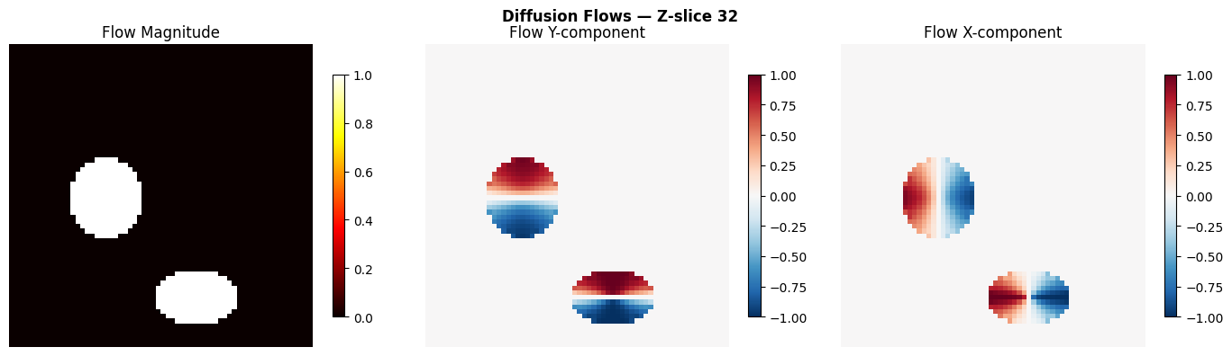
2. Generate Diffusion Flows

The diffusion flow generator solves the heat equation inside each instance, then takes the spatial gradient to produce a flow field that points toward each instance’s topological center.

Since this is the full volume (not a crop from a larger dataset), we pass spatial_mask=None — this uses Dirichlet boundary conditions at the volume edge, keeping flow directed inward.

from topo import generate_diffusion_flows

flows = generate_diffusion_flows(
    gt_instances,
    n_iter=200,
    spatial_mask=None,  # full volume — real boundary
)
print(f"Flow shape: {flows.shape}  (3 x D x H x W)")
print(f"Flow dtype: {flows.dtype}")

Flow shape: (3, 64, 64, 64)  (3 x D x H x W)
Flow dtype: float32

# Visualize flow magnitude and direction at mid-Z
mid_z = gt_instances.shape[0] // 2
fg = gt_instances > 0

flow_mag = np.sqrt((flows ** 2).sum(axis=0))

fig, axes = plt.subplots(1, 3, figsize=(14, 4))

# Flow magnitude
ax = axes[0]
im = ax.imshow(flow_mag[mid_z], cmap="hot", interpolation="nearest")
ax.set_title("Flow Magnitude")
ax.axis("off")
plt.colorbar(im, ax=ax, shrink=0.8)

# Flow Y component
ax = axes[1]
im = ax.imshow(flows[1, mid_z], cmap="RdBu_r", vmin=-1, vmax=1, interpolation="nearest")
ax.set_title("Flow Y-component")
ax.axis("off")
plt.colorbar(im, ax=ax, shrink=0.8)

# Flow X component
ax = axes[2]
im = ax.imshow(flows[2, mid_z], cmap="RdBu_r", vmin=-1, vmax=1, interpolation="nearest")
ax.set_title("Flow X-component")
ax.axis("off")
plt.colorbar(im, ax=ax, shrink=0.8)

fig.suptitle(f"Diffusion Flows — Z-slice {mid_z}", fontweight="bold")
fig.tight_layout()
plt.show()

3. Postprocess: Flow Tracking + Clustering

The postprocessing pipeline:

1. Euler integration: each foreground voxel follows the flow for n_steps

2. Convergence clustering: voxels that end up near each other are grouped

3. Small instance filtering: clusters below min_size are removed

from topo import postprocess_single

result = postprocess_single(
    sem_mask=fg,
    flow=flows,
    n_steps=100,
    step_size=1.0,
    convergence_radius=4.0,
    min_size=50,
    group=1,  # convex morphology group
)
print(f"Recovered instances: {result.max()}")
print(f"GT instances: {n_inst}")

Recovered instances: 4
GT instances: 4

# Compare GT vs recovered
fig, axes = plt.subplots(1, 2, figsize=(10, 4))

ax = axes[0]
ax.imshow(gt_instances[mid_z], interpolation="nearest", cmap="nipy_spectral")
ax.set_title(f"Ground Truth ({n_inst} instances)")
ax.axis("off")

ax = axes[1]
ax.imshow(result[mid_z], interpolation="nearest", cmap="nipy_spectral")
ax.set_title(f"Recovered ({result.max()} instances)")
ax.axis("off")

fig.suptitle("Full-Volume Pipeline Result", fontweight="bold")
fig.tight_layout()
plt.show()

Summary

The full-volume pipeline correctly recovers all instances:

Step	Output
Input	Synthetic instance mask (64x64x64, 4 instances)
Diffusion flows	[3, 64, 64, 64] unit vector field
Postprocessing	Instance labels matching GT

For larger volumes that don’t fit in memory, see the Tiled Stitching Tutorial which splits the volume into overlapping sub-crops and stitches the results.