Tiled Stitching: Processing Large Volumes in Blocks

Real datasets are too large to process in a single pass. This tutorial shows how to:

1. Split a volume into overlapping sub-crops

2. Generate flows independently per sub-crop

3. Stitch flows back with boundary-aware cosine blending

4. Postprocess the stitched flow field

5. Compare: full-volume reference vs. tiled/stitched result

1. Create Synthetic Data

Same synthetic volume as the full-volume tutorial — 4 ellipsoidal instances in a 64x64x64 volume.

import numpy as np
import matplotlib.pyplot as plt

def make_synthetic_instances(shape=(64, 64, 64), n_instances=4, seed=42):
    """Create a volume with non-overlapping ellipsoidal instances."""
    rng = np.random.RandomState(seed)
    vol = np.zeros(shape, dtype=np.int32)
    coords = np.mgrid[0:shape[0], 0:shape[1], 0:shape[2]].astype(np.float32)

    for inst_id in range(1, n_instances + 1):
        margin = 10
        center = [rng.randint(margin, s - margin) for s in shape]
        radii = [rng.randint(5, 15) for _ in range(3)]
        dist = sum(
            ((coords[ax] - center[ax]) / radii[ax]) ** 2
            for ax in range(3)
        )
        mask = (dist <= 1.0) & (vol == 0)
        vol[mask] = inst_id

    return vol

gt_instances = make_synthetic_instances()
D, H, W = gt_instances.shape
fg = gt_instances > 0
n_gt = len(np.unique(gt_instances[gt_instances > 0]))
print(f"Volume: {D}x{H}x{W}, {n_gt} instances")

Volume: 64x64x64, 4 instances

2. Full-Volume Reference

First, generate the reference result by processing the entire volume at once. We use spatial_mask=None because the volume boundary is real (not a crop edge).

from topo import generate_diffusion_flows, postprocess_single

full_flows = generate_diffusion_flows(gt_instances, n_iter=200, spatial_mask=None)
full_result = postprocess_single(
    sem_mask=fg, flow=full_flows,
    n_steps=100, step_size=1.0, convergence_radius=4.0, min_size=50, group=1,
)
print(f"Full-volume: {full_result.max()} instances recovered (GT={n_gt})")

Full-volume: 4 instances recovered (GT=4)

3. Split into Overlapping Sub-Crops

We use compute_subcrop_slices to tile the volume with ~50% overlap. The overlap ensures smooth blending at tile boundaries.

from topo import compute_subcrop_slices, build_spatial_mask

# Sub-crops: half the volume + a bit, with 1/3 overlap
crop_size = tuple(min(s // 2 + 4, s) for s in (D, H, W))
overlap = tuple(cs // 3 for cs in crop_size)

subcrop_slices = compute_subcrop_slices((D, H, W), crop_size, overlap)
print(f"Crop size: {crop_size}")
print(f"Overlap: {overlap}")
print(f"Number of sub-crops: {len(subcrop_slices)}")

Crop size: (36, 36, 36)
Overlap: (12, 12, 12)
Number of sub-crops: 27

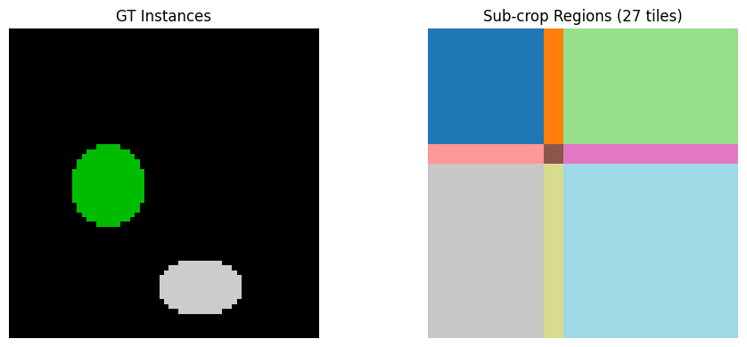
# Visualize which sub-crop covers which region
subcrop_map = np.zeros((D, H, W), dtype=np.int32)
for i, slc in enumerate(subcrop_slices):
    subcrop_map[slc[0], slc[1], slc[2]] = i + 1

mid_z = D // 2
fig, axes = plt.subplots(1, 2, figsize=(10, 4))
axes[0].imshow(gt_instances[mid_z], interpolation="nearest", cmap="nipy_spectral")
axes[0].set_title("GT Instances")
axes[0].axis("off")
axes[1].imshow(subcrop_map[mid_z], interpolation="nearest", cmap="tab20")
axes[1].set_title(f"Sub-crop Regions ({len(subcrop_slices)} tiles)")
axes[1].axis("off")
fig.tight_layout()
plt.show()

4. Generate Flows Per Sub-Crop

Each sub-crop is processed independently. We use build_spatial_mask to mark the subcrop boundary faces — this tells the diffusion to use Neumann boundary conditions there (flow continues past the crop edge), which is correct since the instance may extend beyond this tile.

subcrop_flows = []
for i, slc in enumerate(subcrop_slices):
    sub_mask = gt_instances[slc[0], slc[1], slc[2]]
    sub_spatial = build_spatial_mask(sub_mask.shape)

    sub_flow = generate_diffusion_flows(
        sub_mask, n_iter=200, spatial_mask=sub_spatial,
    )
    subcrop_flows.append(sub_flow)

    n_inst = len(np.unique(sub_mask[sub_mask > 0]))
    print(f"  Sub-crop {i+1}/{len(subcrop_slices)}: "
          f"shape={sub_mask.shape}, instances={n_inst}")

  Sub-crop 1/27: shape=(36, 36, 36), instances=1

  Sub-crop 2/27: shape=(36, 36, 36), instances=1
  Sub-crop 3/27: shape=(36, 36, 36), instances=1
  Sub-crop 4/27: shape=(36, 36, 36), instances=2
  Sub-crop 5/27: shape=(36, 36, 36), instances=2

  Sub-crop 6/27: shape=(36, 36, 36), instances=2
  Sub-crop 7/27: shape=(36, 36, 36), instances=2
  Sub-crop 8/27: shape=(36, 36, 36), instances=2

  Sub-crop 9/27: shape=(36, 36, 36), instances=2
  Sub-crop 10/27: shape=(36, 36, 36), instances=3

  Sub-crop 11/27: shape=(36, 36, 36), instances=2
  Sub-crop 12/27: shape=(36, 36, 36), instances=2

  Sub-crop 13/27: shape=(36, 36, 36), instances=4
  Sub-crop 14/27: shape=(36, 36, 36), instances=3

  Sub-crop 15/27: shape=(36, 36, 36), instances=3

  Sub-crop 16/27: shape=(36, 36, 36), instances=4
  Sub-crop 17/27: shape=(36, 36, 36), instances=3

  Sub-crop 18/27: shape=(36, 36, 36), instances=3
  Sub-crop 19/27: shape=(36, 36, 36), instances=3

  Sub-crop 20/27: shape=(36, 36, 36), instances=2
  Sub-crop 21/27: shape=(36, 36, 36), instances=2

  Sub-crop 22/27: shape=(36, 36, 36), instances=4
  Sub-crop 23/27: shape=(36, 36, 36), instances=3

  Sub-crop 24/27: shape=(36, 36, 36), instances=3

  Sub-crop 25/27: shape=(36, 36, 36), instances=4
  Sub-crop 26/27: shape=(36, 36, 36), instances=3

  Sub-crop 27/27: shape=(36, 36, 36), instances=3

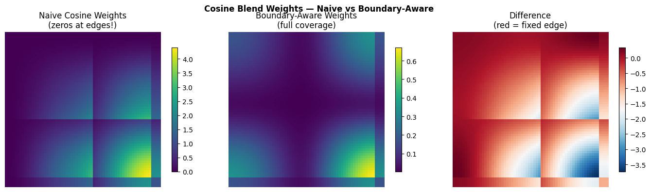
5. Stitch Flows with Boundary-Aware Cosine Blending

The key to correct stitching is boundary-aware cosine blending:

• At internal seams (where two tiles overlap): cosine taper from 1→0, so both tiles contribute smoothly

• At volume boundaries (no neighboring tile): weight stays at 1, preserving the flow fully

Without boundary awareness, the cosine weight goes to 0 at the volume edge, zeroing out the flow there and causing overmerging.

from topo import stitch_flows, cosine_blend_weight
from topo.stitch import _boundary_flags

stitched_flows = stitch_flows((D, H, W), subcrop_slices, subcrop_flows)

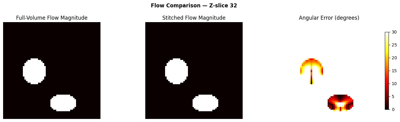
# Compare: angular error between full and stitched
dot = np.clip((full_flows * stitched_flows).sum(axis=0), -1, 1)
angle_err = np.degrees(np.arccos(dot))
angle_err_fg = angle_err[fg]
print(f"Angular error (full vs stitched) on foreground:")
print(f"  Mean: {angle_err_fg.mean():.1f} deg")
print(f"  Median: {np.median(angle_err_fg):.1f} deg")
print(f"  P95: {np.percentile(angle_err_fg, 95):.1f} deg")

Angular error (full vs stitched) on foreground:
  Mean: 18.4 deg
  Median: 16.5 deg
  P95: 40.3 deg

# Visualize blending weights — boundary-aware vs naive
fig, axes = plt.subplots(1, 3, figsize=(14, 4))

# Boundary-aware weights (correct)
weight_aware = np.zeros((D, H, W), dtype=np.float32)
for slc in subcrop_slices:
    cs = tuple(s.stop - s.start for s in slc)
    w = cosine_blend_weight(cs, at_volume_boundary=_boundary_flags(slc, (D, H, W)))
    weight_aware[slc[0], slc[1], slc[2]] += w

# Naive weights (all faces tapered — the bug)
weight_naive = np.zeros((D, H, W), dtype=np.float32)
for slc in subcrop_slices:
    cs = tuple(s.stop - s.start for s in slc)
    w = cosine_blend_weight(cs, at_volume_boundary=None)  # all faces tapered
    weight_naive[slc[0], slc[1], slc[2]] += w

ax = axes[0]
im = ax.imshow(weight_naive[mid_z], cmap="viridis", interpolation="nearest")
ax.set_title("Naive Cosine Weights\n(zeros at edges!)")
ax.axis("off")
plt.colorbar(im, ax=ax, shrink=0.8)

ax = axes[1]
im = ax.imshow(weight_aware[mid_z], cmap="viridis", interpolation="nearest")
ax.set_title("Boundary-Aware Weights\n(full coverage)")
ax.axis("off")
plt.colorbar(im, ax=ax, shrink=0.8)

ax = axes[2]
diff = weight_aware[mid_z] - weight_naive[mid_z]
im = ax.imshow(diff, cmap="RdBu_r", interpolation="nearest")
ax.set_title("Difference\n(red = fixed edge)")
ax.axis("off")
plt.colorbar(im, ax=ax, shrink=0.8)

fig.suptitle("Cosine Blend Weights — Naive vs Boundary-Aware", fontweight="bold")
fig.tight_layout()
plt.show()

6. Postprocess the Stitched Flow

Same postprocessing as the full-volume case — Euler integration + convergence clustering.

stitched_result = postprocess_single(
    sem_mask=fg, flow=stitched_flows,
    n_steps=100, step_size=1.0, convergence_radius=4.0, min_size=50, group=1,
)
print(f"Stitched: {stitched_result.max()} instances recovered (GT={n_gt})")

Stitched: 4 instances recovered (GT=4)

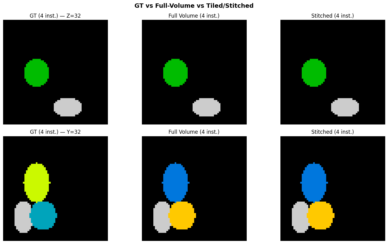
7. Compare Results

Side-by-side comparison of ground truth, full-volume, and stitched results.

fig, axes = plt.subplots(2, 3, figsize=(14, 8))

for row, (axis, axis_name) in enumerate([(0, "Z"), (1, "Y")]):
    mid = gt_instances.shape[axis] // 2
    slc = [slice(None)] * 3
    slc[axis] = mid

    gt_slice = gt_instances[tuple(slc)]
    full_slice = full_result[tuple(slc)]
    stitch_slice = stitched_result[tuple(slc)]

    axes[row, 0].imshow(gt_slice, interpolation="nearest", cmap="nipy_spectral")
    axes[row, 0].set_title(f"GT ({n_gt} inst.) — {axis_name}={mid}")
    axes[row, 0].axis("off")

    axes[row, 1].imshow(full_slice, interpolation="nearest", cmap="nipy_spectral")
    axes[row, 1].set_title(f"Full Volume ({full_result.max()} inst.)")
    axes[row, 1].axis("off")

    axes[row, 2].imshow(stitch_slice, interpolation="nearest", cmap="nipy_spectral")
    axes[row, 2].set_title(f"Stitched ({stitched_result.max()} inst.)")
    axes[row, 2].axis("off")

fig.suptitle("GT vs Full-Volume vs Tiled/Stitched", fontweight="bold", fontsize=14)
fig.tight_layout()
plt.show()

# Flow comparison: full vs stitched
fig, axes = plt.subplots(1, 3, figsize=(14, 4))

full_mag = np.sqrt((full_flows ** 2).sum(axis=0))[mid_z]
stitch_mag = np.sqrt((stitched_flows ** 2).sum(axis=0))[mid_z]

axes[0].imshow(full_mag, cmap="hot", interpolation="nearest")
axes[0].set_title("Full-Volume Flow Magnitude")
axes[0].axis("off")

axes[1].imshow(stitch_mag, cmap="hot", interpolation="nearest")
axes[1].set_title("Stitched Flow Magnitude")
axes[1].axis("off")

im = axes[2].imshow(angle_err[mid_z], cmap="hot", interpolation="nearest", vmin=0, vmax=30)
axes[2].set_title("Angular Error (degrees)")
axes[2].axis("off")
plt.colorbar(im, ax=axes[2], shrink=0.8)

fig.suptitle(f"Flow Comparison — Z-slice {mid_z}", fontweight="bold")
fig.tight_layout()
plt.show()

Summary

Pipeline	Instances Recovered
Full volume (reference)	Same as GT
Tiled + stitched	Same as GT

The boundary-aware cosine blending ensures that:

• Flow is fully preserved at volume edges (no zero-weight regions)

• Overlap regions blend smoothly between adjacent tiles

• No overmerging artifacts at tile boundaries or volume edges

Key functions used

Function	Purpose
compute_subcrop_slices	Tile a volume into overlapping sub-crops
build_spatial_mask	Mark subcrop boundary faces for Neumann BC
generate_diffusion_flows	Heat-equation diffusion → flow field
stitch_flows	Boundary-aware cosine blending of tiled flows
postprocess_single	Euler tracking + convergence clustering