Minimal Tutorial

DaCapo is a framework for easy application of established machine learning techniques on large, multi-dimensional images.

Needed Libraries for this Tutorial

For the tutorial we will use data from the skimage library, and we will use matplotlib to visualize the data. You can install these libraries using the following commands:

pip install 'scikit-image[data]'
pip install matplotlib

Introduction and overview

In this tutorial we will cover the basics of running an ML experiment with DaCapo.

DaCapo has 4 major configurable components:

1. dacapo.datasplits.DataSplit

2. dacapo.tasks.Task

3. dacapo.architectures.Architecture

4. dacapo.trainers.Trainer

These are then combined in a single dacapo.experiments.Run that includes your starting point (whether you want to start training from scratch or continue off of a previously trained model) and stopping criterion (the number of iterations you want to train).

Environment setup

If you have not already done so, you will need to install DaCapo. You can do this by first creating a new environment and then installing DaCapo using pip.

conda create -n dacapo python=3.10
conda activate dacapo

Then, you can install DaCapo using pip, via GitHub:

pip install git+https://github.com/janelia-cellmap/dacapo.git

pip install dacapo-ml

Be sure to select this environment in your Jupyter notebook or JupyterLab.

Config Store

Configs, model checkpoints, stats, and snapshots can be saved in:

• a local folder

• an S3 bucket

• a MongoDB server

To define where the data goes, create a dacapo.yaml configuration file either in ~/.config/dacapo/dacapo.yaml or in ./dacapo.yaml. Here is a template:

type: files
runs_base_dir: /path/to/my/data/storage

Alternatively, you can define it by setting an environment variable: DACAPO_OPTIONS_FILE=/PATH/TO/MY/DACAPO_FILES.

The runs_base_dir defines where your on-disk data will be stored. The type setting determines the database backend. The default is files, which stores the data in a file tree on disk. Alternatively, you can use mongodb to store the data in a MongoDB database. To use MongoDB, you will need to provide a mongodbhost and mongodbname in the configuration file:

mongodbhost: mongodb://dbuser:dbpass@dburl:dbport/
mongodbname: dacapo

# First we need to create a config store to store our configurations
import multiprocessing

# This line is mostly for MacOS users to avoid a bug in multiprocessing
multiprocessing.set_start_method("fork", force=True)
from dacapo.store.create_store import create_config_store, create_stats_store

config_store = create_config_store()

/opt/hostedtoolcache/Python/3.10.15/x64/lib/python3.10/site-packages/tqdm/auto.py:21: TqdmWarning: IProgress not found. Please update jupyter and ipywidgets. See https://ipywidgets.readthedocs.io/en/stable/user_install.html
  from .autonotebook import tqdm as notebook_tqdm

Creating FileConfigStore:
	path: /home/runner/dacapo/configs

Data Preparation

DaCapo works with zarr, so we will download skimage example cell data and save it as a zarr file.

import numpy as np
from funlib.geometry import Coordinate, Roi
from funlib.persistence import prepare_ds
from scipy.ndimage import label
from skimage import data
from skimage.filters import gaussian

# Download the data
cell_data = (data.cells3d().transpose((1, 0, 2, 3)) / 256).astype(np.uint8)

# Handle metadata
offset = Coordinate(0, 0, 0)
voxel_size = Coordinate(290, 260, 260)
axis_names = ["c^", "z", "y", "x"]
units = ["nm", "nm", "nm"]

# Create the zarr array with appropriate metadata
cell_array = prepare_ds(
    "cells3d.zarr/raw",
    cell_data.shape,
    offset=offset,
    voxel_size=voxel_size,
    axis_names=axis_names,
    units=units,
    mode="w",
    dtype=np.uint8,
)

# Save the cell data to the zarr array
cell_array[cell_array.roi] = cell_data

# Generate and save some pseudo ground truth data
mask_array = prepare_ds(
    "cells3d.zarr/mask",
    cell_data.shape[1:],
    offset=offset,
    voxel_size=voxel_size,
    axis_names=axis_names[1:],
    units=units,
    mode="w",
    dtype=np.uint8,
)
cell_mask = np.clip(gaussian(cell_data[1] / 255.0, sigma=1), 0, 255) * 255 > 30
not_membrane_mask = np.clip(gaussian(cell_data[0] / 255.0, sigma=1), 0, 255) * 255 < 10
mask_array[mask_array.roi] = cell_mask * not_membrane_mask

# Generate labels via connected components
labels_array = prepare_ds(
    "cells3d.zarr/labels",
    cell_data.shape[1:],
    offset=offset,
    voxel_size=voxel_size,
    axis_names=axis_names[1:],
    units=units,
    mode="w",
    dtype=np.uint8,
)
labels_array[labels_array.roi] = label(mask_array.to_ndarray(mask_array.roi))[0]

print("Data saved to cells3d.zarr")
import zarr

print(zarr.open("cells3d.zarr").tree())

Data saved to cells3d.zarr
/
 ├── labels (60, 256, 256) uint8
 ├── mask (60, 256, 256) uint8
 └── raw (2, 60, 256, 256) uint8

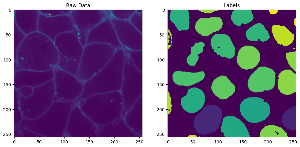
Here we show a slice of the raw data:

# a custom label color map for showing instances
import matplotlib.pyplot as plt

fig, axes = plt.subplots(1, 2, figsize=(12, 6))

# Show the raw data
axes[0].imshow(cell_array.data[0, 30])
axes[0].set_title("Raw Data")

# Show the labels using the custom label color map
axes[1].imshow(labels_array.data[30])
axes[1].set_title("Labels")

plt.show()

Datasplit

Where can you find your data? What format is it in? Does it need to be normalized? What data do you want to use for validation?

We have already saved some data in cells3d.zarr. We will use this data for training and validation. We only have one dataset, so we will be using the same data for both training and validation. This is not recommended for real experiments, but is useful for this tutorial.

from dacapo.experiments.datasplits.simple_config import SimpleDataSplitConfig
from funlib.geometry import Coordinate

datasplit_config = SimpleDataSplitConfig(name="cells3d", path="cells3d.zarr")
datasplit = datasplit_config.datasplit_type(datasplit_config)
config_store.store_datasplit_config(datasplit_config)

datasplit = datasplit_config.datasplit_type(datasplit_config)
# viewer = datasplit._neuroglancer()

config_store.store_datasplit_config(datasplit_config)

Task

What do you want to learn?

• Instance Segmentation: Identify and separate individual objects within an image.

• Affinities: Learn the likelihood of neighboring pixels belonging to the same object.

• Distance Transform: Calculate the distance of each pixel to the nearest object boundary.

• Foreground/Background: Distinguish between object pixels and background pixels.

Each of these tasks is commonly learned and evaluated with specific loss functions and evaluation metrics. Some tasks may also require specific non-linearities or output formats from your model.

from dacapo.experiments.tasks import DistanceTaskConfig, AffinitiesTaskConfig

resolution = 260  # nm
# an example distance task configuration
# note that the clip_distance, tol_distance, and scale_factor are in nm
dist_task_config = DistanceTaskConfig(
    name="example_dist",
    channels=["cell"],
    clip_distance=resolution * 10.0,
    tol_distance=resolution * 10.0,
    scale_factor=resolution * 20.0,
)
# if the config already exists, delete it first
# config_store.delete_task_config(dist_task_config.name)
config_store.store_task_config(dist_task_config)

# an example affinities task configuration
affs_task_config = AffinitiesTaskConfig(
    name="example_affs",
    neighborhood=[(1, 0, 0), (0, 1, 0), (0, 0, 1)],
)
# config_store.delete_task_config(dist_task_config.name)
config_store.store_task_config(affs_task_config)

Architecture

The setup of the network you will train. Biomedical image to image translation often utilizes a UNet, but even after choosing a UNet you still need to provide some additional parameters. How much do you want to downsample? How many convolutional layers do you want?

from dacapo.experiments.architectures import CNNectomeUNetConfig

# Note we make this UNet 2D by defining kernel_size_down, kernel_size_up, and downsample_factors
# all with 1s in z meaning no downsampling or convolving in the z direction.
architecture_config = CNNectomeUNetConfig(
    name="example_unet",
    input_shape=(2, 132, 132),
    eval_shape_increase=(8, 32, 32),
    fmaps_in=2,
    num_fmaps=8,
    fmaps_out=8,
    fmap_inc_factor=2,
    downsample_factors=[(1, 4, 4), (1, 4, 4)],
    kernel_size_down=[[(1, 3, 3)] * 2] * 3,
    kernel_size_up=[[(1, 3, 3)] * 2] * 2,
    constant_upsample=True,
    padding="valid",
)
config_store.store_architecture_config(architecture_config)

Trainer

How do you want to train? This config defines the training loop and how the other three components work together. What sort of augmentations to apply during training, what learning rate and optimizer to use, what batch size to train with.

from dacapo.experiments.trainers import GunpowderTrainerConfig

trainer_config = GunpowderTrainerConfig(
    name="example",
    batch_size=10,
    learning_rate=0.0001,
    num_data_fetchers=1,
    snapshot_interval=1000,
    min_masked=0.05,
    clip_raw=False,
)
config_store.store_trainer_config(trainer_config)

Run

Now that we have our components configured, we just need to combine them into a run and start training. We can have multiple repetitions of a single set of configs in order to increase our chances of finding an optimum.

from dacapo.experiments import RunConfig
from dacapo.experiments.run import Run

iterations = 2000
validation_interval = iterations // 4
run_config = RunConfig(
    name="example_run",
    datasplit_config=datasplit_config,
    task_config=affs_task_config,
    architecture_config=architecture_config,
    trainer_config=trainer_config,
    num_iterations=iterations,
    validation_interval=validation_interval,
    repetition=0,
)
config_store.store_run_config(run_config)

Retrieve Configurations

All of the configurations are saved in the config store. You can retrieve them as follows:

• Architectures: These define the network architectures used in your experiments.

architectures = config_store.retrieve_architecture_configs()

• Tasks: These specify the tasks that your model will learn, such as instance segmentation or affinity prediction.

tasks = config_store.retrieve_task_configs()

• Trainers: These configurations define how the training process is conducted, including parameters like batch size and learning rate.

trainers = config_store.retrieve_trainer_configs()

• Datasplits: These configurations specify how your data is split into training, validation, and test sets.

datasplits = config_store.retrieve_datasplit_configs()

• Runs: These combine all the above configurations into a single experiment run.

runs = config_store.retrieve_run_configs()

Train

NOTE: The run stats are stored in the runs_base_dir/stats directory. You can delete this directory to remove all stored stats if you want to re-run training. Otherwise, the stats will be appended to the existing files, and the run won’t start from scratch. This may cause errors.

from dacapo.train import train_run

# from dacapo.validate import validate
from dacapo.experiments.run import Run

from dacapo.store.create_store import create_config_store

config_store = create_config_store()

run = Run(config_store.retrieve_run_config("example_run"))
if __name__ == "__main__":
    train_run(run)

Creating FileConfigStore:
	path: /home/runner/dacapo/configs

Starting/resuming training for run example_run...
Creating FileStatsStore:
	path    : /home/runner/dacapo/stats
Trained until 2000, but validated until 2001! Deleting extra validation stats
Current state: trained until 2000/2000
Creating local weights store in directory /home/runner/dacapo
Resuming training from iteration 2000
Retrieving weights for run example_run, iteration 2000

Trained until 2000. Finished.

Visualize

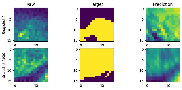
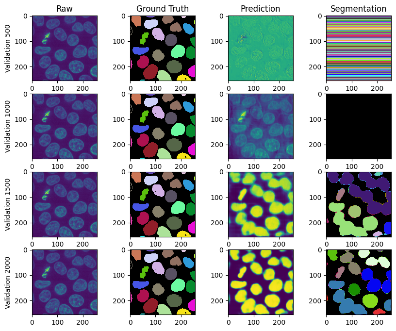
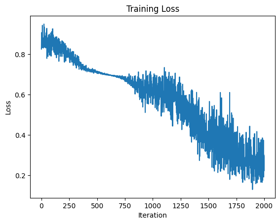
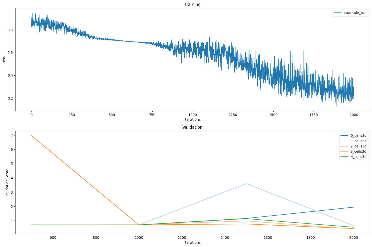
Let’s visualize the results of the training run. DaCapo saves a few artifacts during training including snapshots, validation results, and the loss.

stats_store = create_stats_store()
training_stats = stats_store.retrieve_training_stats(run_config.name)
stats = training_stats.to_xarray()
print(stats)
plt.plot(stats)
plt.title("Training Loss")
plt.xlabel("Iteration")
plt.ylabel("Loss")
plt.show()

Creating FileStatsStore:
	path    : /home/runner/dacapo/stats
<xarray.DataArray (iterations: 2000)>
array([0.7177695 , 0.71814048, 0.71345633, ..., 0.22248204, 0.165636  ,
       0.10437805])
Coordinates:
  * iterations  (iterations) int64 0 1 2 3 4 5 ... 1994 1995 1996 1997 1998 1999

from dacapo.plot import plot_runs

plot_runs(
    run_config_base_names=[run_config.name],
    validation_scores=["voi"],
    plot_losses=[True],
)

# # other ways to visualize the training stats
# stats_store = create_stats_store()
# training_stats = stats_store.retrieve_training_stats(run_config.name)
# stats = training_stats.to_xarray()
# plt.plot(stats)
# plt.title("Training Loss")
# plt.xlabel("Iteration")
# plt.ylabel("Loss")
# plt.show()

Creating FileConfigStore:
	path: /home/runner/dacapo/configs
Creating FileStatsStore:
	path    : /home/runner/dacapo/stats

import zarr
from matplotlib.colors import ListedColormap

np.random.seed(1)
colors = [[0, 0, 0]] + [list(np.random.choice(range(256), size=3)) for _ in range(254)]
label_cmap = ListedColormap(colors)

run_path = config_store.path.parent / run_config.name

# BROWSER = False
num_snapshots = run_config.num_iterations // run_config.trainer_config.snapshot_interval

if num_snapshots > 0:
    fig, ax = plt.subplots(num_snapshots, 3, figsize=(10, 2 * num_snapshots))

    # Set column titles
    column_titles = ["Raw", "Target", "Prediction"]
    for col in range(3):
        ax[0, col].set_title(column_titles[col])

    for snapshot in range(num_snapshots):
        snapshot_it = snapshot * run_config.trainer_config.snapshot_interval
        # break
        raw = zarr.open(f"{run_path}/snapshot.zarr/{snapshot_it}/volumes/raw")[:]
        target = zarr.open(f"{run_path}/snapshot.zarr/{snapshot_it}/volumes/target")[0]
        prediction = zarr.open(
            f"{run_path}/snapshot.zarr/{snapshot_it}/volumes/prediction"
        )[0]
        c = (raw.shape[2] - target.shape[1]) // 2
        ax[snapshot, 0].imshow(raw[1, raw.shape[0] // 2, c:-c, c:-c])
        ax[snapshot, 1].imshow(target[target.shape[0] // 2])
        ax[snapshot, 2].imshow(prediction[prediction.shape[0] // 2])
        ax[snapshot, 0].set_ylabel(f"Snapshot {snapshot_it}")
    plt.show()

# # %%
# Visualize validations
import zarr

num_validations = run_config.num_iterations // run_config.validation_interval
fig, ax = plt.subplots(num_validations, 4, figsize=(10, 2 * num_validations))

# Set column titles
column_titles = ["Raw", "Ground Truth", "Prediction", "Segmentation"]
for col in range(len(column_titles)):
    ax[0, col].set_title(column_titles[col])

for validation in range(1, num_validations + 1):
    dataset = run.datasplit.validate[0].name
    validation_it = validation * run_config.validation_interval
    # break
    raw = zarr.open(f"{run_path}/validation.zarr/inputs/{dataset}/raw")
    gt = zarr.open(f"{run_path}/validation.zarr/inputs/{dataset}/gt")
    pred_path = f"{run_path}/validation.zarr/{validation_it}/{dataset}/prediction"
    out_path = f"{run_path}/validation.zarr/{validation_it}/{dataset}/output/WatershedPostProcessorParameters(id=2, bias=0.5, context=(32, 32, 32))"
    output = zarr.open(out_path)[:]
    prediction = zarr.open(pred_path)[0]
    c = (raw.shape[2] - gt.shape[1]) // 2
    if c != 0:
        raw = raw[:, :, c:-c, c:-c]
    ax[validation - 1, 0].imshow(raw[1, raw.shape[1] // 2])
    ax[validation - 1, 1].imshow(
        gt[gt.shape[0] // 2], cmap=label_cmap, interpolation="none"
    )
    ax[validation - 1, 2].imshow(prediction[prediction.shape[0] // 2])
    ax[validation - 1, 3].imshow(
        output[output.shape[0] // 2], cmap=label_cmap, interpolation="none"
    )
    ax[validation - 1, 0].set_ylabel(f"Validation {validation_it}")
plt.show()